49  Stationarity and Differencing

49.1 Understanding stationarity

Definition

‘Stationarity’ means that the statistical properties of a time-series are consistent over time. This implies that the mean, variance, and covariance of the series remain unchanged no matter at what point in time we observe them.

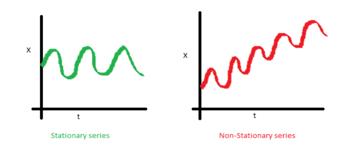
The figure in green below is stationary; the one in red is non-stationary.

Importance

  • Stationarity is really important in time-series analysis, because it allows for the application of various statistical modeling techniques that assume this property. When a time series is stationary, it means that its behavior is predictable and therefore can be modeled.

  • Many statistical models, such as ARIMA (Autoregressive Integrated Moving Average), are based on the premise that the time series is stationary.

Type One: Strict stationarity

‘Strict stationarity’ is a stringent form of stationarity.

It means that the statistical properties of the time series - its mean, variance, and also all higher moments (like skewness and kurtosis) - must be invariant over time.

Type Two: Weak/Covariance stationarity

‘Weak’, or ‘covariance stationarity’ is a less stringent version and more commonly used in time series analysis. It requires that a time series must have a constant mean and variance, and that its covariance should only depend on the lag between observations and not the actual time at which the observations were taken.

Imagine a daily temperature record that fluctuates around a long-term average; while day-to-day temperatures vary, their overall distribution does not change drastically over years. This form of stationarity is more realistic and commonly encountered in real-world data.

Illustration

Consider a dataset of monthly unemployment rates. If this data is ‘weakly stationary’, the average rate and the variability in rates from month to month remain constant over years, and the relationship between the rate in one month and the next (regardless of whether it’s January to February or July to August) stays consistent.

Conversely, a strict stationary series would imply that these rates, along with all aspects of their distribution, do not change at all over time, a scenario less likely to occur in real economic data.

49.2 Characteristics

Constant mean

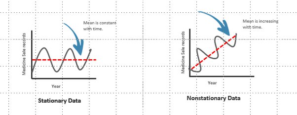
  • A stationary time series has a constant mean over time.
  • Regardless of when you observe the series, its average value does not show a discernible trend or systematic change.

Note that the series fluctuates around a stable, horizontal average line, not showing trends upwards or downwards over the long term.

Constant variance

Another crucial attribute of stationarity is constant variance. This means the fluctuations or spread of the time series data around the mean remains uniform over time.

  • Imagine a calm sea with waves of relatively the same height over days; similarly, a stationary time series exhibits fluctuations of consistent amplitude.

  • In graphical terms, the series would display a consistent band of fluctuation around the mean, without periods of significant tightening or widening of the range.

Autocovariance

The third key feature of stationary time series is consistent autocovariance.

  • Autocovariance measures the relationship between different values in the series at different times, depending on the lag or the time interval between them.

  • In a stationary series, this relationship is not dependent on the time at which the data is observed but only on the lag. For instance, the correlation between sales figures in one month and the next should remain similar whether we’re looking at data from January to February or from June to July.

49.3 Testing for stationarity

Visual inspection

The first approach to test for stationarity is through visual inspection, using time series plots.

  • This involves graphically plotting the time series data to look for signs of a constant mean, variance, and no recurring patterns that depend on time.

  • If a plot shows an oscillating pattern but hovering around a constant mean and with uniform amplitude of fluctuations, it suggests stationarity.

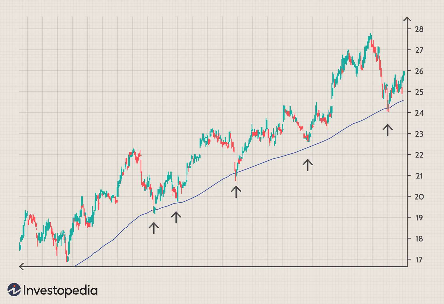
  • Conversely, trends, seasonal patterns, or changing variances in the plot indicate non-stationarity.

The Augmented Dickey-Fuller (ADF) Test

We can also test for stationarity by using various statistical tests.

  • One of the most commonly used is the Augmented Dickey-Fuller (ADF) test. It specifically tests for the presence of a unit root, a condition implying non-stationarity.

  • A small p-value (typically < 0.05) suggests that the null hypothesis of a unit root (i.e., non-stationarity) can be rejected, confirming that the time series is stationary.

(see also Kwiatkowski-Phillips-Schmidt-Shin (KPSS) and Phillips-Perron (PP) tests).

Examples

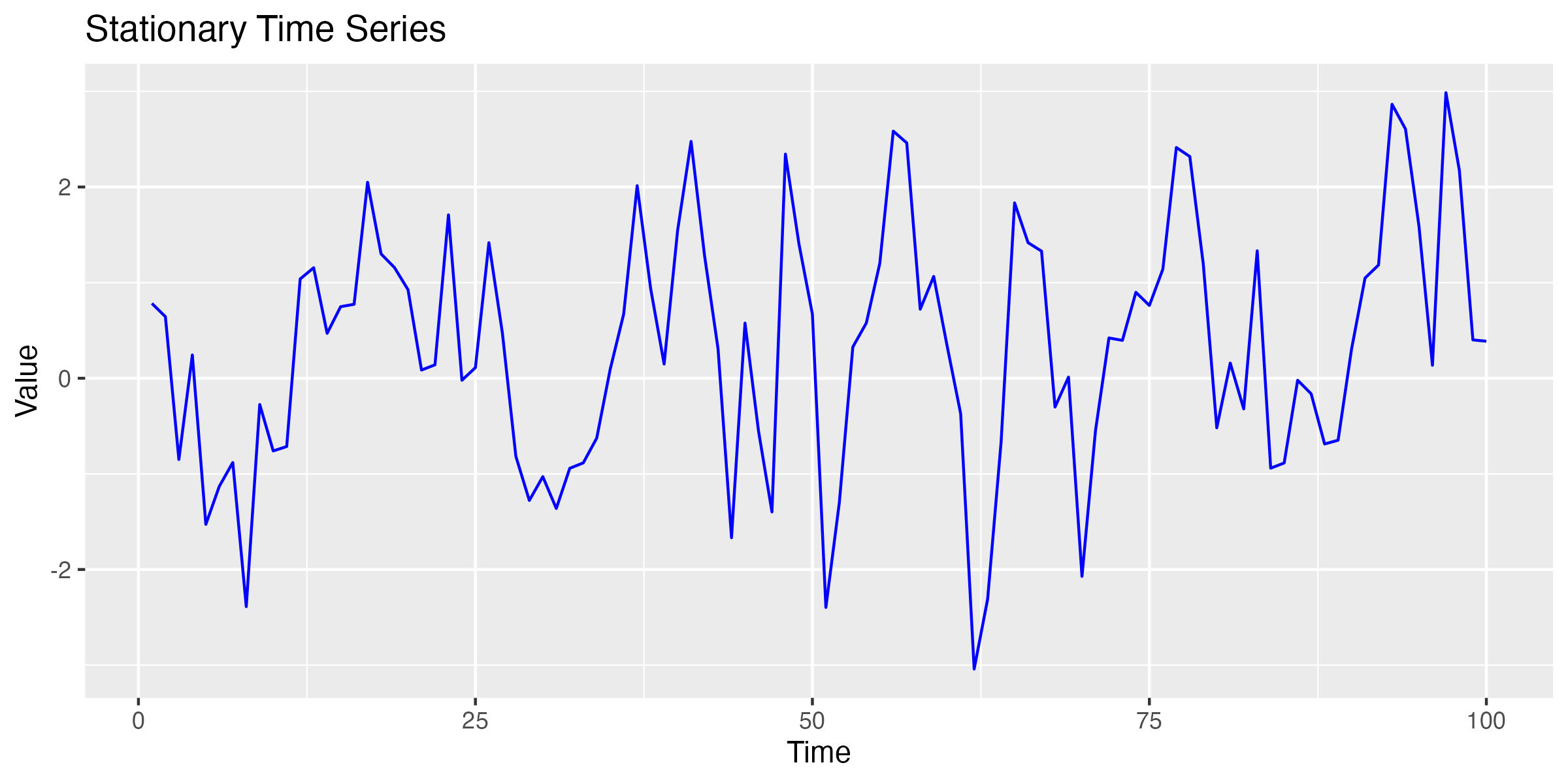
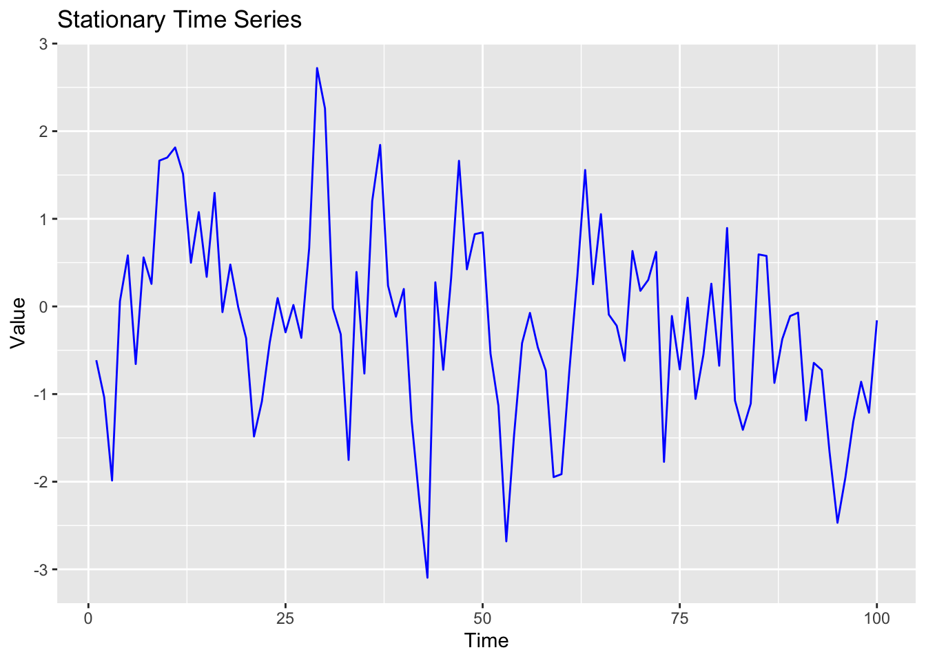
In the first example, I have created a time series that is stationary.

Note that the resulting plot confirms the stationary pattern described above, and that the p-value of the ADF is < 0.05, suggesting that we can reject the null hypothesis and confirm the data is stationary.

Show code for stationary data
# Load libraries
library(forecast)
library(ggplot2)
library(tseries)

# Function to generate a stationary time series
generate_stationary_ts <- function(n) {
  arima.sim(model = list(ar = 0.5), n = n)
}

# Generate time series data
stationary_ts <- generate_stationary_ts(100)

# Plot the time series
p <- ggplot() + geom_line(aes(x = 1:100, y = stationary_ts), color = "blue") +
     ggtitle("Stationary Time Series") +
     xlab("Time") + ylab("Value")
print(p)

Show code for stationary data
# Conduct Augmented Dickey-Fuller Test
adf_test <- adf.test(stationary_ts, alternative = "stationary")

# Output the result of the ADF test
print(adf_test)

    Augmented Dickey-Fuller Test

data:  stationary_ts
Dickey-Fuller = -4.6665, Lag order = 4, p-value = 0.01
alternative hypothesis: stationary

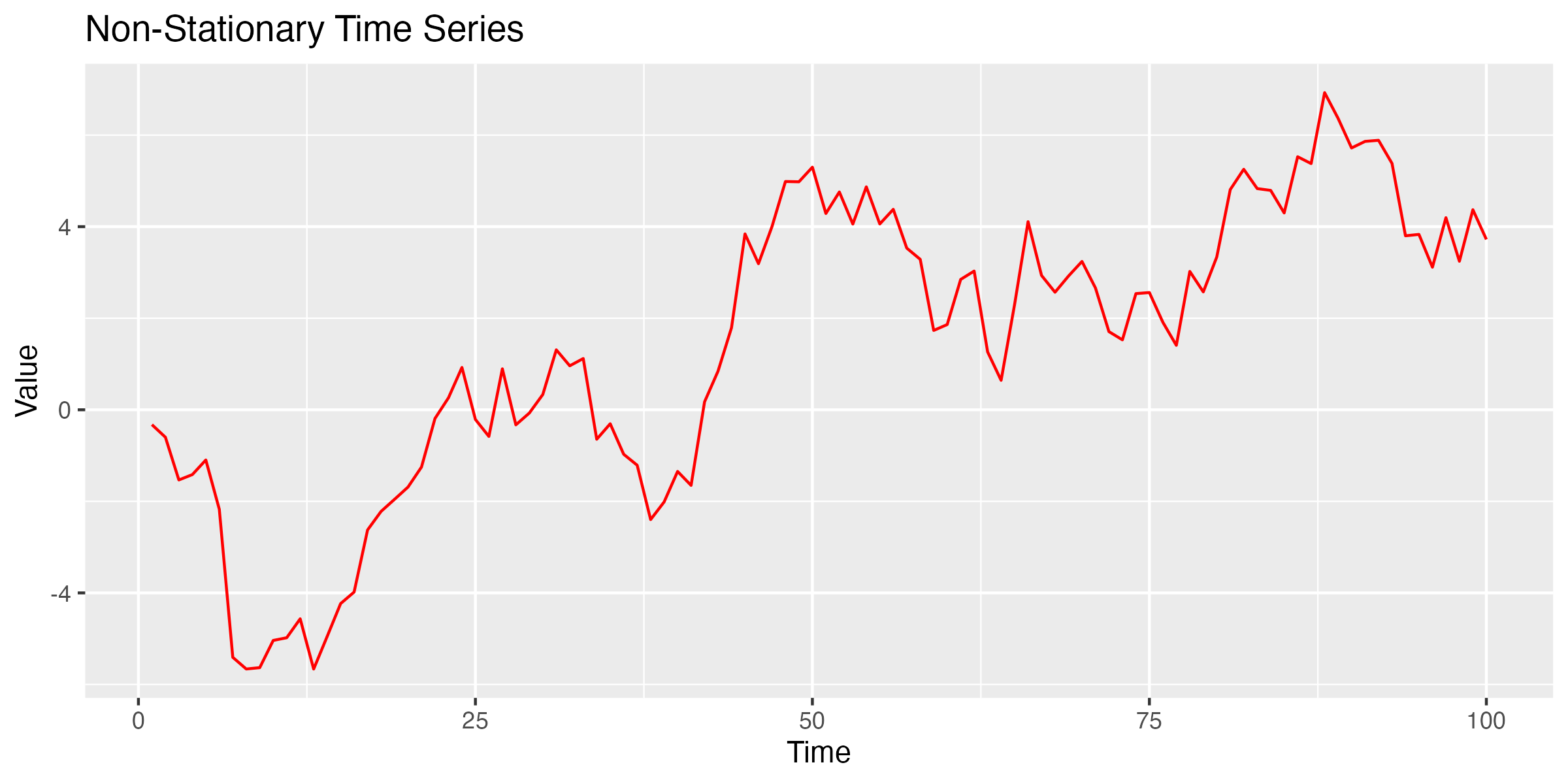
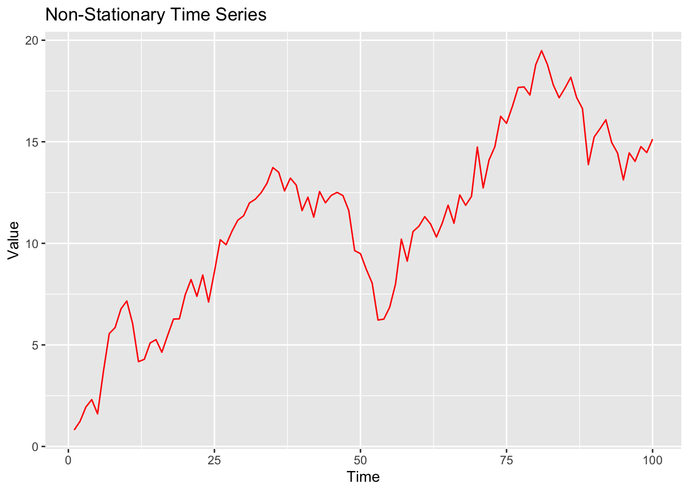
Now, I will create another data set that is non-stationary, and apply the same processes to it.

  • Note the visual pattern with clear trends, and that the p-value of the ADF is > 0.05.
Show code for non-stationary data
# Load libraries
library(forecast)
library(ggplot2)
library(tseries)

# Function to generate a non-stationary time series
generate_non_stationary_ts <- function(n) {
  cumsum(rnorm(n))
}

# Generate time series data
non_stationary_ts <- generate_non_stationary_ts(100)

# Plot the time series
p <- ggplot() + geom_line(aes(x = 1:100, y = non_stationary_ts), color = "red") +
     ggtitle("Non-Stationary Time Series") +
     xlab("Time") + ylab("Value")
print(p)

Show code for non-stationary data
# Conduct Augmented Dickey-Fuller Test
adf_test <- adf.test(non_stationary_ts, alternative = "stationary")

# Output the result of the ADF test
print(adf_test)

    Augmented Dickey-Fuller Test

data:  non_stationary_ts
Dickey-Fuller = -2.5571, Lag order = 4, p-value = 0.3459
alternative hypothesis: stationary

49.4 Transforming non-stationary data

We’ve made the point that stationarity is an important feature of time series data if we want to do further exploration of the data.

If in our initial exploration of the data we find that it is non-stationary, we can use number of different techniques to address this, and convert it to stationary.

Differencing

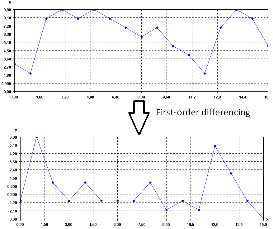
‘Differencing’ can be used to transform a non-stationary time series into a stationary one.

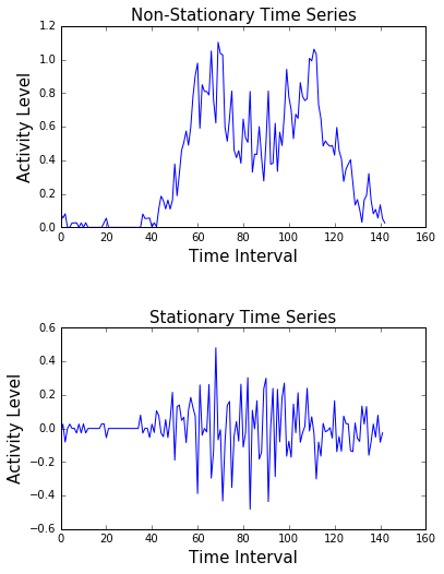
It involves subtracting the current value of the series from the previous value (first-order differencing), as in the following figure:

For example, if we have a timeseries of monthly sales data showing an increasing trend (hence, non-stationary), differencing this data by subtracting each month’s sales from the previous month’s can help stabilise the mean.

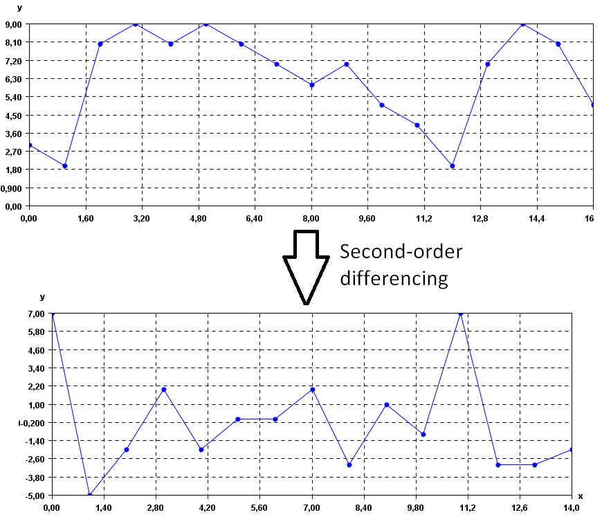
If the trend or seasonality is not removed in the first difference, a second differencing (as above) might be needed.

Imagine you’re tracking the number of steps you take each day. On Monday, you take 3000 steps, on Tuesday 3500, and on Wednesday 4000. The number of steps is increasing each day, which is a trend.

In differencing, instead of looking at the total steps each day, you look at how much the number of steps changes from one day to the next. So, instead of the original numbers (3000, 3500, 4000), you look at the differences (500 on Tuesday from Monday, 500 on Wednesday from Tuesday). This new series of differences (500, 500) is your ‘differenced’ series.

Log transformation

Differencing is effective for addressing trends (non-stationarity) in data.

Another technique, ‘log transformation’, is especially useful for stabilising the variance of a time-series.

Imaginer you’re looking at the money you save each week. Some weeks you save a little, like £10, and other weeks a lot more, like £100 or £1000. This wide range of values can make it hard to see patterns or trends in your savings behaviour.

By applying a log transformation, you’re essentially ‘squishing’ this wide range of values into a narrower, more manageable scale. When you take the logarithm of your savings, smaller amounts and larger amounts get closer together in value.

For instance, the logarithm (usually base 10 is used) of £10 is 1, of £100 is 2, and of £1000 is 3. Now, instead of dealing with £10, £100, and £1000, you’re dealing with 1, 2, and 3, which are easier to compare and analyse.
By applying a logarithmic scale to each data point in the series, large values are scaled down, and the variance becomes more constant.

  • For instance, consider a company’s revenue data that grows exponentially over time.

  • Applying a log transformation can help in reducing the scaling effect, making the data more suitable for analysis.

This method is most effective when dealing with data that exhibit exponential growth.